pid-simulation-with-micro800_Fig 1



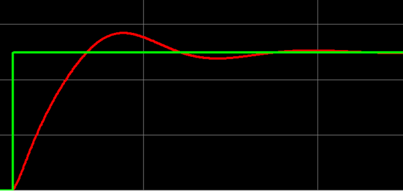
This is a simplified application designed to simulate the behavior of a process variable that can be connected to a PID controller. The application includes executable files that enable this simulation in Connected Components Workbench (CCW) for Micro800 controllers.
pid-simulation-with-micro800_Fig 1

Downloads
Please note: You will need to agree to the Terms & Conditions for each download.

Need Help?
If you need help with an application or have feedback from the Innovation Center, please contact us.
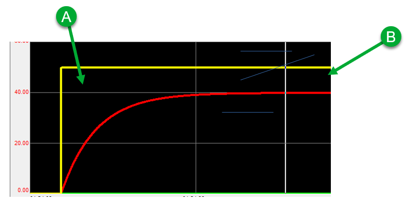
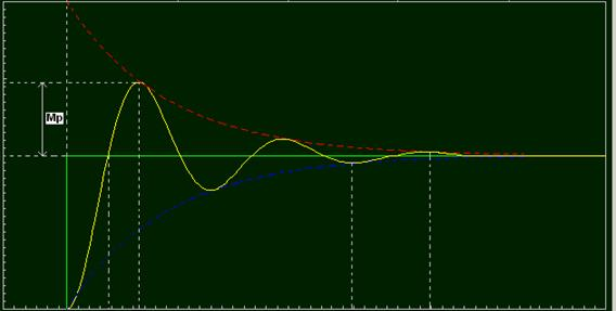
In CCW, there is no built-in Lead-Lag function that would allow us to simulate a process with behavior similar to that shown in the following image, therefore, the simulation will be implemented by constructing a first-order filter, as described in the following steps.
| A | Phase lag (Lag) |
| B | Steady-state error |
pid-simulation-with-micro800_Fig 2
This application can be used in CCW with Micro800 controllers. It allows users to understand the effects of PID gains and various configuration parameters, as well as simulate simple processes for demonstration purposes or virtual commissioning.
How can I make it work?
Requirements: products, tools, prior knowledge.

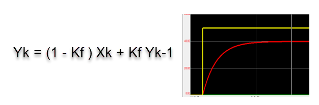
In the case of CCW, the Phase Lead-Lag instruction is not available; therefore, the code will be written to implement a first-order filter based on the following equation:
pid-simulation-with-micro800_Fig 3
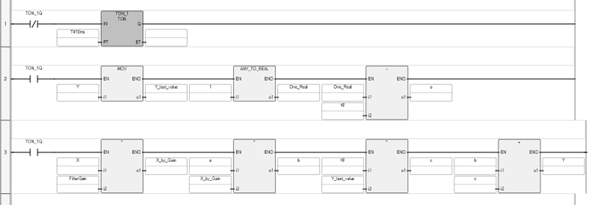
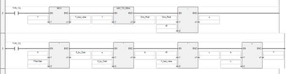
Insert the following code in Ladder Logic.
Since this first-order filter operates as a function of time, the TON timer provides the trigger required to perform the filter calculations.
For this application, we recommend using a timer value of 10 ms, although this value can be adjusted according to the dynamics of the process being simulated.
pid-simulation-with-micro800_Fig 4
The remaining blocks perform the arithmetic operations required to implement the filter equation. In this application, variable “X” represents the input variable, and variable “Y” represents the output variable (both tags are of the Real data type).
For this example, which uses a 10 ms execution time, we recommend using a gain value of Kf = 0.993. However, this value can be adjusted according to the process being simulated.
pid-simulation-with-micro800_Fig 5
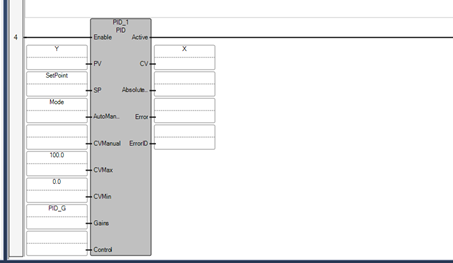
Add a PID function. Configure tag “Y” as the PID input (PV) and tag “X” as the PID output (CV).
pid-simulation-with-micro800_Fig 6
Adjust the parameters and gains according to the process being simulated.
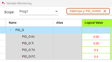
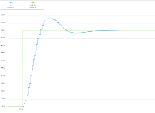
To obtain a response similar to the one shown in the following image, it is recommended to use the following gain values:
pid-simulation-with-micro800_Fig 7
pid-simulation-with-micro800_Fig 8
With this parameterization, it is possible to achieve the behavior of an underdamped system with approximately 20% overshoot and stabilization within three half-cycles.
However, the parameters can be adjusted to obtain any desired response according to the process being simulated.
pid-simulation-with-micro800_Fig 9
PID Simulation with Micro800
Version 2.0 - October 2026
